Monte Carlo Simulation in Stock Analysis: A Beginner's Guide

What is Monte Carlo Simulation?

Monte Carlo simulation is a probabilistic modeling technique that uses random sampling to estimate possible outcomes of an uncertain event. In stock analysis, it helps investors understand the range of potential returns and risks by simulating thousands of possible future scenarios.

Named after the famous Monte Carlo Casino, this method relies on randomness to explore all possible outcomes—just like rolling dice in a casino.

Why Use Monte Carlo in Stock Analysis?

Traditional valuation methods (like DCF) provide a single-point estimate of a stock's value. However, the future is uncertain, and key variables—such as revenue growth, profit margins, and discount rates—can vary widely.

Monte Carlo simulation addresses this uncertainty by:

  • Modeling key variables as probability distributions (e.g., revenue growth could range between 3% and 10%).
  • Running thousands of simulations to generate a distribution of possible outcomes.
  • Providing probabilistic insights (e.g., "There’s a 70% chance the stock will return at least 8% annually").
  • How Monte Carlo Works in Stock Valuation

    Step 1: Define Key Variables and Their Distributions

    Monte Carlo starts by identifying the uncertain variables that impact a stock's value. Common variables include:

    | Variable | Description | Example Distribution |

    |-----------------------|-------------------------------------------------------------------------------------------------|--------------------------------|

    | Revenue Growth Rate | Annual percentage increase in revenue. | Normal (μ=5%, σ=2%) |

    | Operating Margin | Operating income as a percentage of revenue. | Triangular (min=10%, mode=15%)|

    | Discount Rate (WACC) | Weighted average cost of capital—used to discount future cash flows to present value. | Uniform (6%–10%) |

    | Terminal Growth Rate | Long-term growth rate after the forecast period. | Uniform (1%–4%) |

    Step 2: Run Thousands of Simulations

    For each simulation:

  • A random value is drawn from each variable’s probability distribution.
  • These values are plugged into a DCF model to calculate the stock’s intrinsic value.
  • The process is repeated 10,000 times (or more) to generate a distribution of possible outcomes.
  • Step 3: Analyze the Results

    The output of a Monte Carlo simulation is a distribution of returns, which can be visualized as a histogram. This distribution helps investors answer questions like:

    • What is the expected return of this stock?
    • What is the probability of a positive return?
    • What is the worst-case scenario (downside risk)?

    Why 10,000 Simulations?

    Running 10,000 simulations may seem excessive, but it serves two critical purposes:

  • Statistical Significance: More simulations reduce the margin of error and provide a smoother, more reliable distribution of outcomes.
  • Tail Risk Coverage: Extreme scenarios (e.g., market crashes or hypergrowth) are rare but impactful. 10,000 simulations ensure these "tail events" are adequately represented.
  • How to Read a Monte Carlo Return Distribution

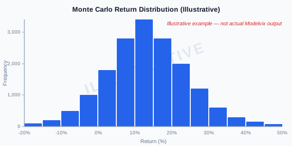
    A Monte Carlo histogram shows the frequency of possible returns. Here’s how to interpret it:

    !Monte Carlo Histogram Example

    • X-axis (Return %): The range of possible returns (e.g., -20% to +50%).
    • Y-axis (Frequency): The number of simulations that resulted in a specific return range.
    • Peak of the Histogram: The most likely return range (e.g., 8%–12%).
    • Left Tail: Represents downside risk (e.g., returns below -10%).
    • Right Tail: Represents upside potential (e.g., returns above 30%).

    Key Metrics to Focus On

  • Expected Return (Mean): The average return across all simulations.
  • Median Return (P50): The middle value of the distribution—50% of simulations fall above or below this return.
  • Probability of Positive Return: The percentage of simulations where the return is greater than 0%.
  • Downside Risk (P5): The worst-case return in the bottom 5% of simulations (e.g., -15%).
  • Example: Monte Carlo for Tesla (TSLA)

    Let’s simulate Tesla’s (TSLA) stock returns using Monte Carlo:

    • Revenue Growth: Normal distribution (μ=15%, σ=5%).
    • Operating Margin: Triangular distribution (min=8%, mode=12%, max=18%).
    • WACC: Uniform distribution (7%–11%).
    • Terminal Growth: Uniform distribution (1%–3%).

    Results after 10,000 simulations:

    • Expected Return: 12.4%
    • Probability of Positive Return: 78%
    • Downside Risk (P5): -8.2%
    • Upside Potential (P95): +35.6%

    Interpretation:

    • There’s a 78% chance Tesla will generate a positive return.
    • The worst-case scenario (bottom 5%) is a -8.2% loss.
    • The best-case scenario (top 5%) is a +35.6% gain.

    Advantages of Monte Carlo Simulation

  • Quantifies Uncertainty: Provides a range of possible outcomes rather than a single-point estimate.
  • Reveals Tail Risks: Highlights extreme scenarios that traditional models might miss.
  • Improves Decision-Making: Helps investors assess risk-reward trade-offs more effectively.
  • Flexible and Adaptable: Can incorporate complex variables and dependencies (e.g., correlation between revenue growth and margins).
  • Limitations of Monte Carlo

  • Garbage In, Garbage Out (GIGO): The quality of the output depends on the quality of the input distributions.
  • Assumption-Dependent: Results are sensitive to the chosen probability distributions.
  • Computationally Intensive: Requires significant computational power for large-scale simulations.
  • Not a Crystal Ball: Cannot predict the future—only estimates possible outcomes based on historical data and assumptions.
  • How to Use Monte Carlo in Your Investment Process

  • Run a Monte Carlo simulation for your target stock.
  • Analyze the return distribution to understand expected returns and risks.
  • Compare with your risk tolerance—does the downside risk align with your comfort level?
  • Combine with other metrics (e.g., P/E, ROIC) for a holistic view.
  • Monitor over time to track changes in risk and return expectations.
  • Conclusion

    Monte Carlo simulation is a powerful tool for quantifying uncertainty in stock analysis. By running thousands of scenarios, it provides a probabilistic view of potential returns and risks, helping investors make more informed decisions.

    Key takeaway: Monte Carlo doesn’t predict the future, but it helps you prepare for it by revealing the range of possible outcomes.

    ---

    Disclaimer: This content is for educational purposes only and does not constitute financial advice. Always conduct your own research before making investment decisions.