What Is a Monte Carlo Analysis? Simulation for Stocks
What is Monte Carlo Simulation?
Monte Carlo simulation is a probabilistic modeling technique that uses random sampling to estimate possible outcomes of an uncertain event. In stock analysis, it helps investors understand the range of potential returns and risks by simulating thousands of possible future scenarios.
Named after the famous Monte Carlo Casino, this method relies on randomness to explore all possible outcomes—just like rolling dice in a casino.
Source: NIST — Monte Carlo Tool
Why Use Monte Carlo in Stock Analysis?
Traditional valuation methods (like DCF) provide a single-point estimate of a stock's value. However, the future is uncertain, and key variables—such as revenue growth, profit margins, and discount rates—can vary widely.
Monte Carlo simulation addresses this uncertainty by:
New to the DCF side of this approach? Start with our introduction to DCF and Monte Carlo simulation.
Prefer a structured, step-by-step lesson? Take our interactive lesson: Monte Carlo Simulation in Stock Valuation.
How Monte Carlo Works in Stock Valuation
Step 1: Define Key Variables and Their Distributions
Monte Carlo starts by identifying the uncertain variables that impact a stock's value. Common variables include:
| Variable | Description | Example Distribution |
|---|---|---|
| Revenue Growth Rate | Annual percentage increase in revenue. | Normal (μ=5%, σ=2%) |
| Operating Margin | Operating income as a percentage of revenue. | Triangular (min=10%, mode=15%) |
| Discount Rate (WACC) | Weighted average cost of capital—used to discount future cash flows to present value. | Uniform (6%–10%) |
| Terminal Growth Rate | Long-term growth rate after the forecast period. | Uniform (1%–4%) |
Step 2: Run Thousands of Simulations
For each simulation:
Step 3: Analyze the Results
The output of a Monte Carlo simulation is a distribution of returns, which can be visualized as a histogram. This distribution helps investors answer questions like:
- What is the expected return of this stock?
- What is the probability of a positive return?
- What is the worst-case scenario (downside risk)?
Why 10,000 Simulations?
Running 10,000 simulations may seem excessive, but it serves two critical purposes:
How to Read a Monte Carlo Return Distribution
A Monte Carlo histogram shows the frequency of possible returns. Here’s how to interpret it:
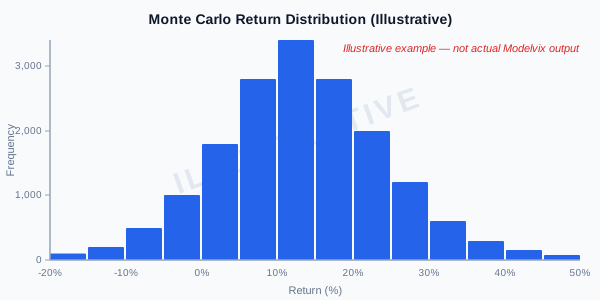
Illustrative example — not actual Modelvix output.
- X-axis (Return %): The range of possible returns (e.g., -20% to +50%).
- Y-axis (Frequency): The number of simulations that resulted in a specific return range.
- Peak of the Histogram: The most likely return range (e.g., 8%–12%).
- Left Tail: Represents downside risk (e.g., returns below -10%).
- Right Tail: Represents upside potential (e.g., returns above 30%).
Key Metrics to Focus On
For a practical, step-by-step guide to reading a Monte Carlo histogram, see How to Read a Monte Carlo Histogram.
Example: Monte Carlo for Tesla (TSLA)
Let’s simulate Tesla’s (TSLA) stock returns using Monte Carlo:
Note: The following Tesla simulation inputs and outputs are illustrative parameters designed to demonstrate distribution modeling in Modelvix. They are not actual Modelvix simulation results.
- Revenue Growth: Normal distribution (μ=15%, σ=5%).
- Operating Margin: Triangular distribution (min=8%, mode=12%, max=18%).
- WACC: Uniform distribution (7%–11%).
- Terminal Growth: Uniform distribution (1%–3%).
Results after 10,000 simulations:
- Expected Return: 12.4%
- Probability of Positive Return: 78%
- Downside Risk (P5): -8.2%
- Upside Potential (P95): +35.6%
Interpretation:
- There’s a 78% chance Tesla will generate a positive return.
- The worst-case scenario (bottom 5%) is a -8.2% loss.
- The best-case scenario (top 5%) is a +35.6% gain.
Advantages of Monte Carlo Simulation
Limitations of Monte Carlo
How to Use Monte Carlo in Your Investment Process
Conclusion
Monte Carlo simulation is a powerful tool for quantifying uncertainty in stock analysis. By running thousands of scenarios, it provides a probabilistic view of potential returns and risks, helping investors make more informed decisions.
Key takeaway: Monte Carlo doesn’t predict the future, but it helps you prepare for it by revealing the range of possible outcomes.
---
Disclaimer: This content is for educational purposes only and does not constitute financial advice. Always conduct your own research before making investment decisions.